

Financial Management: Pricing
Post 3 in the series on management: pricing theory & tactics

In the previous post, I explained how to decompose revenue growth into its constituent parts: volume (change in the quantity of products/services sold), pricing (changes in product prices) and mix (changes in the relative volume of the different kinds of products sold). In this post, I will explain how to determine the optimal price to charge for a product, and then I will discuss different ways to set prices, or use mix to increase average price/product.
The first section is a bit theory-heavy, and I imagine not all that interesting to most people; if you’re not into microeconomics, I suggest you skip to the second section, which (I think) is also interesting for anyone who wants to understand how companies set prices and how they play around with different pricing tactics. These tactics can be used in many different industries — from service provision to FMCG — , though not at all (e.g. it’s hard to imagine certain kind of promotions in the car industry!)
You may have heard that companies set prices by taking their costs and adding a surcharge on it; while it’s true that many companies do this, this practice is a terrible, terrible idea: there is no reason to suggest that this way of setting prices maximises profit (not to mention that it completely fails to take into account the consumer). Instead, here is how serious companies set prices.
Optimal Price — Theory
If you’ve been to business school or studied microeconomics, you will have probably heard that the optimal price is the one that makes marginal revenue equal to marginal cost. I will start by explaning this theory (as it’s not necessarily intuitive), I will then show how to apply in practice, and will finally discuss some of its limitations.
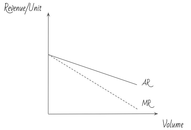
Let’s start with the concepts of average and marginal revenue per unit sold. Average revenue (AR) is, as you’d expect, equal to total revenue divided by number of units sold; marginal revenue (MR) refers to the additional revenue generated by selling one more unit (but it is not, as we will see in a minute, the additional revenue that unit generates itself!). Both of these slope downwards, with MR < AR:

Average revenue slopes downwards because to sell more units you need to set a lower price; so by definition, the more units you sell, the lower the average price. The reason MR is < AR is harder to wrap one’s head around: as mentioned above, MR is the additional revenue generated by selling one more unit. But this is not equal to the price of the last unit sold! It is easier to understand the reason for this using an example:
Let’s say you are selling 10 chocolate bars a month for $2. Then, your average revenue per bar is $2. If you want to increase the quantity of bars to 11, you will need to lower your price (and hence your average revenue/bar), say to $1.9. Now, it’s true you are going to make $1.9 for the 11th bar you sell; but at the same time, you are going to lose $0.1 for the 10 bars you had already been selling. So, your marginal revenue is
= $1.9 — $0.1 x 10 = $0.9
(This is a convoluted way of getting to this answer; the simpler thing to do is to notice that at the $2 price point, your total revenue is 10 bars x $2 = $20; at the $1.9 price point, your total revenue is 11 bars x $1.9 = $20.9. The difference between the two ($0.9) is the marginal revenue).
Similarly, we can plot the curves for the average and marginal cost of producing the units we sell. These curves look very different, depending on the actual costs involved in manufacturing and selling the products. The kind of cost function I will be using in this post assumes a fixed cost of production (say, the salaries of the employees at a factory, which you need to pay regardless of how many products you make) and a constant variable cost (e.g. the raw materials of the product). Other cost functions include those that have only constant variable costs (e.g. if you do not own a factory, but outsource production instead) or those that have rising or declining variable costs (I think the case of rising variable costs is rarer, but it could happen if your production relies on a rare raw material; as you use more of it, you might drive up its market price). A cost function that involves a fixed cost and a stable marginal cost can be plotted as follows:

The marginal cost / unit is shown as a straight line, since it does not change depending on volume; the average cost per unit starts at infinity (this is just a mathematical quirk, because average cost is defined as Total Cost / Volume; when volume is 0, this fraction is undefinable) and approaches the marginal cost as volume increases (this is because as volume increases, fixed cost / volume becomes smaller and smaller, so for very large volumes, average cost is only a tiny bit higher than MC).
Merging the charts for cost and revenue, we get:

What I hope is self-evident is that a firm is profitable as long as its average revenue is higher than its average cost — so, in the chart above, the firm is profitable as long as it sells between Q1 and Q2 units (and charges between P1 and P3).
What is less obvious is that this firm makes maximum profit when it charges P2, selling Q2 units; this is the point where marginal revenue is equal to marginal cost. For most people, this is not intuitive: why would profit be highest when marginal revenue and cost are equal? Surely profit should be higher then marginal revenue is higher than marginal cost?
Not so. Think of it this way: if marginal revenue is higher than marginal cost, the firm should reduce the price it charges, because the revenue it will make by doing so and selling an additional unit will be higher than the cost it will incur by producing that unit. So this is how you set the optimal price: it’s the price that makes your marginal revenue equal to your marginal cost. But it bears repeating that this does not mean you should set a price equal to marginal cost, because marginal revenue is not equal to the latest price.
(In case you’re into maths, you can prove this algebraically. To maximise profit, you want to find to find the value of x that results in the highest possible value for the equation TR(x) — TC(x) [where TR = total revenue, TC = total cost].
If you were to plot profit, i.e. TR(x) — TC(x), the resulting chart would look like a concave curve. This is because at point zero on the x-axis (so the point where the firm sells no products at all), profit is also zero (or negative, if the firm has fixed costs); and to get very large values of x (i.e. to sell a very large quantity of products), the firm must charge a very low price, so profit will again decline. It logically follows that there must be some values of x for which profit goes up, and then some values for which it goes back down. Hence a concave curve.
You may remember from your maths classes that to find the maximum point of a concave curve, you need to find the value of x for which the derivative of the curve is equal to zero. You may also remember that the definition of a curve’s derivative is the curve’s rate of change — in other words, its marginal value. So, to find the point at which profit is maximised, we take the derivative of TR(x) — TC(x):
d(TR(x) — TC(x))/dx = MR(x) — MC(x).
If you are interested in this stuff, I recommend Microeconomics for Managers, by David Kreps.)
Optimal Price — Practice
Of course, in practice, when you show up at work no-one will hand you a neat demand and cost curve. After all, these curves are not constant: on the cost side, variable costs fluctuate all the time, as the price of various commodities and utilities used in production changes daily. On the revenue side, demand for a product at a given price depends on the prices of competitors’ products, substitutes, and complements. And, trust me on this, if you walk into a meeting and start talking about derivatives, you will be laughed out of the room.
So in practice, what you do is you model price changes from the current price level:

In the example above, a company sells 100 units of a product for $10; it costs $6 to make each product. Note that we only take variable cost into account here: the company has to pay its fixed costs regardless of how many products it manufactures, so we can exclude them from the calculation.
The model (which you can find here) suggests that if the company lowers the price of the product to $9, it will sell 40 more units. As a result, its revenue will increase by $260; its costs will also go up, as it needs to manufacture 40 more units — hence, profit will increase by $20.
What if the firm decreases the price to $8, and sells another 40 units as a result? It turns out that doing this will actually decrease profit:
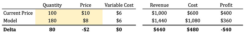
This seems to suggest that $9 is the optimal price.
Of course, the difficulty lies in guessing how many units the firm will sell if the price changes. Companies try to make an intelligent guess based on a number of different pieces of evidence, which include:
Past experience: how did volume respond to changes in price in the past?
Competitive products: have competitors changed their prices recently? What happened to their volumes? (in some industries, it is easy to get this data — for instance, there are companies that aggregate Point-Of-Sale data from different retailers and sell it back to manufacturers; in other instances, a company can approximate their competitors’ volumes by looking at their own. For example, if a competitor lowers their price, and your volume drops by 20 units, it is reasonable to assume that the two are related :))
Market research & experimentation: some companies run trials, commission surveys, conduct experiments etc.
At P&G I had a wealth of external and internal data I could use to make such decisions; still, as mentioned above, past data is not always reliable: for example, I could not always use the fact that a particular product had changed prices before, because competitors had changed their prices in the meantime. So, my preference was to avoid point-estimates, and rely on sensitivity analyses instead. A sensitivity analysis shows how a combination of variables affects a particular measure; in the case of pricing, I would produce a table showing the profit change resulting from different price and quantity combinations; this way, I could tell what volume uplift was required to increase profit for any given price. I would share this with the sales teams, and we would use it to make our pricing decisions. I will show how to do sensitivity analysis in a future post.
There’s one more thing missing from this model. Few companies produce a single product, and many of a company’s products are often substitutes to an extent. Hence, changing the price of one product might affect the volume of another. This is called cannibalisation; I will discuss multi-product offerings at the end of this post, and in more detail in a future post.
Different ways to change a product’s price
Changing the retail (aka list) price of a product is only one possible way to change a product’s price. Other approaches include:
Changing the size of a product while keeping its price constant;
Running promotions; there are different kinds of promotions, mainly price cuts, two-for-one (aka buy one, get one free) type deals, or x for $y — each of which will be covered seperately below;
Playing with mix and loyalty schemes.
(This list is not exhaustive; there may be other pricing tactics that I have not considered — for example, auctions. Feel free to suggest others in the comments.)
I will first give a quick description for each of the above, and will then share a model that can be used to make pricing decisions.
First, a quick table summarising the advantages and disadvantages of the various approaches:

Sizing
One way of changing a product’s price is to change the quantity of a product contained in a unit, while keeping the unit’s price constant. For example, suppose your company makes and sells shampoo bottles. If you are currently selling 100ml bottles for $10, then if you want to take pricing, what you can do is switch to selling a slightly smaller bottle, say a 90ml one, for the same price. Similarly, if you want to decrease the price, you can fill the bottle with 110ml instead. The financials of the decision look like this:

A couple of things to note here:
Consider the price increase through sizing: given that total revenue did not change, it sounds strange to claim that this is a real price increase; in fact, according to the table above, the benefits seem to stem from a cost decrease, rather than a price increase. But, if we use shampoo quantity rather than number of bottles as the measure for volume, and following the logic outlined in the previous post in the series, we can see that this decision leads to a negative $100 volume impact, and a positive $100 pricing impact. The reconciliation below helps clarify the situation:

This model assumes that the cost/bottle is directly proportional to the bottle size. In reality, this is probably not the case: though it’s true that the cost of the raw materials of the shampoo itself will be so, the cost of the packaging (i.e. the bottle itself) won’t change, unless we shrink it too.
The assumes that we will sell the same number of bottles in all scenarios. This may not be true: consumers may notice the price/ml increase and switch brands (and, understandably, they might find this tactic dishonest compared to a list price increase, which would harm the brand’s image — a good example of this in practice was when Toblerone changed the shape of their chocolate). On the other hand, assuming their actual consumption of shampoo does not change, consumers may buy more bottles so that they end up consuming the same ml of shampoo over a certain period.
Notice that price increases are more profitable through LP changes, whereas sizing is more profitable when it comes to price decreases (as long as the number of units sold is the same in both cases).
(Addendum: after I had published this post, a friend reminded me that reducing price through sizing has an additional marketing benefit: increasing size by 50% allows you to make a claim such as ‘now 50% more product’ or something along these lines — and so, the big, impressive number 50 sticks to consumers’ minds; but in fact, a 50% size increase is equal to a 33% price decrease, which sounds less impressive.)
Promotions: Temporary Price Cuts
This one is pretty simple: you offer a discount on a product for a limited period of time by reducing its price. I am not going to reproduce a model for this, as for all intents and purposes the financials look exactly the same as in Figure 5 — the difference being that the effect is temporary.
This is a good place to expand a little on the advantages of running promotions instead of reducing the list price:
As the promotion only runs for a short period of time, the average price of the product for the whole year is higher than it would be if the company reduced the list price. This is a good way for a company to do price discrimination: consumers who are very price-sensitive will wait for the product to be on offer, and will purchase it then; such consumers might not buy the product at all if no discounts were offered. However, consumers who do not care about the price all that much will buy it at list price. If the company reduced the list price, it would be leaving money on the table.
Promotions can unlock what is known as premium display — both in-store, where retailers offer better shelf space to promoted products, and online, where online marketplaces might feature promoted products on the homepage.
Consumers get a kick out of buying products on sale. Though I haven’t looked at studies while writing this post, I think I recall reading about experiments where consumers were more likely to buy a product with an ‘on offer’ sticker than the same product at the same price sans sticker. In fact, unscrupulous companies sometimes mark up prices just before bringing them back down, claiming that their producs are now on sale (though many countries have regulations to prevent this — for instance, in the UK, retailers can only claim a product is on offer if it has been selling for a higher price for a certain number of weeks beforehand).
Finally, price cuts can induce some consumers to try a product, who will then be convinced to pay the full price when the promotion period runs out (companies often achieve the same objective by using coupons, or offering trial-sized products (think of the 5ml fragrance sachets you sometime find in fashion magazines), but it is difficult to run such initiatives at large scale).
Promotions: 2 for 1 (buy one, get one free)
This kind of promotion is equivalent to a 50% price cut, but has some advantages over it:
Not all consumers will notice the promotion and take advantage of it. When you offer a price cut, every single product you sell will have the discount applied at checkout; but with a 2f1 deal, if consumers do not add a second product to their basket, they will pay full price for the product they do buy. Hence, the so-called Volume Sold On Deal is lower for 2f1 offers than for price cuts. (VSOD is usually expressed a a %; e.g. 30% VSOD means that 30% of the product units bought by consumers had discount applied to them.)
At worst, a 2f1 deal is exactly equivalent to a price-cut; at best, however, it generates more revenue and profit.
Whether or not a 2f1 deal is better than a price cut depends on consumer behaviour, which determines what will happen to the number of products sold when the product is on offer. Consider the following example: suppose our firm currently sells 100 products for $10 each, thus generating $1,000 in revenue. If you then run a 50% price cut, your revenue will be $500 (assume no volume change for now). The effect of a 2f1 deal, on the other hand, varies in each of the following three scenarios (which are not exhaustive):
If the 100 products are bought by 100 different consumers, each of whom buy one product, and all of whom decide to take advantage of the offer, then when we run our promotion we will sell 200 units, still making $1,000 in revenue (though incurring higher costs, as we need to manufacture double the number of products).
If the 100 products are bought by 50 consumers, each of whom buys 2 products, then the effect of our promotion will be exactly the same as the 50% price cut. (If it is true that our promotion will not get us new consumers, then it is a very stupid promotion to run).
If things play out as in the first scenario above, but we also induce 100 new consumers to take advantage of the offer and buy the product, then we will sell 400 products (200 consumers buying 2 products each), generating $2,000 in revenue; note that this is again better than a price cut, even if a price cut also induces 100 new consumers to buy the product.

Note that in this example, all promotions are less profitable than selling at list price; still, 2f1 is always at least as profitable as an equivalent the price cut (assuming that the two tactics will have similar volume effects; it could be that a price cut would induce more conusmers to try the product than the 2f1 promo would, because of the lower cash outlay).
(Note that here I show the price as $5 for the 2f1 deal; this is because 100 units are offered at $10, and 100 at $0 — hence ending up with an average price of $5. This is not the best way to model this — I will share a more sophisticated model that can be used for all kinds of deals later on.)
Here’s another way to think about why 2f1 deals are more profitable: a product has a different cost to the consumer than it has to the retailer. To the consumer, it makes no difference whether they are offered more product or an equivalent price cut; to the retailer, the two are different, because the cost of the product is less.
(Clearly, the chief difficulty here is guessing how consumers to respond to the promotion; as mentioned in the previous section, companies can use past data or other pieces of evidence to estimate this. But an additional concern is that it is not sufficient to understand how volume will respond during the promotional period, but what will happen to it in subsequent periods: for example, suppose we run the promotion for one month, and it plays out as in the first scenario above. What this tells us is that over this month, our revenue would be the same regardless of whether we run the promotion or not. But if these consumers buy one product every month, and the product does not expire within a month, then what we will see is 0 revenue the month following the promotion. This kind of effect is very, very difficult to capture, unless we can identify specific users and track their behaviour over time (though easier to do with e-commerce).)
2f1 deals also have two disadvantages over price cuts:
I said ealier that it makes no difference to the consumer whether they are offered more product, or an equivalent price cut; this is true in terms of cost per quantity of product, but not true in terms of cash outlay. We humans are not always perfectly rational; paying $1 for 1 product may feel cheaper than paying $2 for 2 products. Moreover, some consumers are cash-constrained, so they would rather minimise their immediate cash expense. For this reason, price cuts are some times more appealing, and are better for driving penetration (a term that denotes % of consumers who have bought a particular product over a certain period) and trial.
Price cuts are more flexible. You can offer a 25% or 30% price cut; you cannot do that with a 2f1-type deal (or rather, you can, but in more convoluted ways (e.g. 3f2) that are not quite as effective, marketing-wise).
Promotions: x for $y
In this kind of promotion, consumers can choose to buy either a single product at its listed price, or a higher quantity of products for a lower average price per product. For example, if you are selling a product for $10, you can run a promotion where consumers can buy two units of the product for $18. This is equivalent to a 10% discount, as the average price for the product if $9. Here’s an example of the deal:

The advantages of this deal over 2f1-type deals is:
It will almost certainly have a lower VSOD, as the deal is not quite as attractive. You might think that I’m not comparing like-for-like here: I am saying this deal is better, yet this is not an effect of the deal’s mechanism, but of the resulting promo price. True, but the point is that using this kind of deal, you can still secure premium display, and a fancy “10% off” sticker (or pop up), without having to offer the deal to all consumers; in other words, your actual average discount is lower than the promotional discount; you get the financial benefit of the former, with the marketing benefits of the latter.
They are more flexible in terms of getting to a specific price/product.
Finally, pushing more volume (whether it is via sizing, 2f1 or x for $y) has one additional benefit: it blocks competitive promotions in future periods. If consumers buy two packs of your toothpaste because they are on promotion, they do not need to buy more, even if your competitors also run deals next week. (Thanks to ND who reminded me of this!)
A better model
The models I shared for calculating the promotion and price cut impacts are a bit too simplistic — they do not show all variables one needs. A better model needs to allow you as the analyst to change all relevant variables in one go. Here’s an example of such a model (which you can find here, and start using right away :)):

A few comments on this:
For the model to work correctly, you need to set a measure of quantity; for example, if you are selling shampoo, this could be ml; if you are selling nappies, it could be nappies per pack. For some businesses, units are sold in quantities of 1 by default (e.g. airline tickets, unless you are offering packages) — that’s fine, the model is still usable.
In the example above, sizing has exactly the same effect as 2f1, because I modelled the effect of doubling the quantity of the product contained in a unit. Generally, sizing is more flexible in that you can adjust it more easily; however, sizing is also more permanent, as it may require packaging changes, new procedures in factories etc.
I have assumed no change in the number of units sold, except for the ‘mechanical’ uplift. Another way to think of this is that the model assumes consumers will only buy more products in order to take advantage of the deal. I’ve also kept the oversimplified assumptions discussed above.
The 2f1 deal has a 50% VSOD, with a 0 promo price; in other words, the model interprets the deal as ‘the first product is sold at full price, the second at zero — hence, 50% of the products are on deal’. Notice that this assumes all consumers will take advantage of the deal; if we think some consumers will not notice the deal, and hence only buy one product, we need to lower the VSOD (but also the number of units sold) (if you want, you can build even more sophisticated models, with seperate inputs for number of consumers and quantity bought by consumer).
Mix & Loyalty schemes
Companies can opt to change the average price for a product through mix or various loyalty schemes. Though not outright pricing, these tactics are, in my view, the best ways of increasing profitability. This is because they are flexible, transparent, fair, and allow for price discrimination — i.e. they allow companies to get closer to charging every consumer what they are willing to pay.
I will focus here on mix, because the concept is basically the same for loyalty scheme. The difference is that loyalty schemes can be even more targetted than mix, they have the benefit of collecting user data, and are more likely to induce consumers to buy again from you.
The idea behind mix is offering a product that is very similar to your existing one, but with some additional features that justify a price increase. By offering both products, you get to keep your price-conscious consumers, who will buy the cheaper one, while also increasing average price by ‘trading-up’ the less price-sensitive ones. Here’s an example of how you can model the financials for mix:

Suppose you want to increase the price of a product. Then, if you just increase the list price, you will end up selling fewer units — potentially leading to profit loss.
But suppose you launch a new product — e.g. if you are selling shampoo, you might launch a new bottle with a new fragrance, or a 2–in-1 shampoo and conditioner, and sell it at a higher price. Then, according to this model, 50 of your consumers will keep buying the exisitng product, but the other half will try the new one — hence leading to higher profit.
Note that in this example I assumed that the new product costs the same to manufacture as the existing one. In reality, since you need some sort of product enhancement to justify the higher price, this may not be the case. But even if the more premium product has the same gross margin as the basic product (i.e. has the same cost as % of price/ml), it would still be more profitable — I will explain this in more detail in a subsequent post on cost structure.
The possible types of mix are too many to list — but here are three of the most common ones:
Basic-Premium mix: this is the case of the example above, where you offer a slightly better product for a higher price. For example, Always Night is priced at a premium compared to Always Normal (look at the price per pad).
Size mix: price-sensitive consumers often buy in bulk, and so a good way to target them is to offer a discount for larger sizes. For example, Always Night Big Pack has a cheaper price per pad than the Always Night pack above. (Though personally, I have always had a nagging doubt about this in the back of my mind: yes, value-senstitive consumers buy in bulk, but so do loyal consumers, who’d presumably be willing to pay more, and are only buying in bulk for convenience.)
Channel mix: you can charge different prices depending on where you sell your product. It’s not unreasonable to assume that people who shop at Waitrose are less price-sensitive than those who shop at Tesco.
Final Considerations
I mentioned earlier that the theory of optimal pricing has some limitations — well, one, but it’s a big one: it’s not easy determining a product’s marginal cost. In the strictest sense, you should look at the cost of producing one additional product — so far, so good. But how ought one to think about things like R&D or brand marketing costs? They are not exactly variable — you don’t spend more on these for each additional unit you sell; but at the same time, you do need them to sell more units. So what ought you do? Ideally, you’d want to model the Return on Investment (ROI) of the various combinations of levels of marketing and R&D spend, and price/unit. But this is easier said than done — getting reliable ROI data for R&D and brand marketing is extremely hard.
Re pricing tactics, my personal view is that things like changing the price of a product through sizing and promotions can verge on the dishonest. Unfortunately, consumers really, really like promotions — I have seen examples of retailers lowering the list price of a product to a level below its past promo price, and yet achieving fewer unit sales! Changing consumers’ habits is not easy, and as long as people like to feel like they’ve got a bargain — regardless of whether it is true or not, objectively — companies have an incentive to run promotions.
In closing, I will re-iterate that mix and other ways to target different consumers different prices is (in my view) the fairest and best way to increase profitability. Some people object to this notion — the very term ‘price discrimination’ has negative connotations. I struggle with this notion: surely there is nothing wrong with charging more to people who can afford it? Surely it’s fair to charge people what they are willing to pay? But I digress — this series is focused on the technical aspects of running a business, rather than business ethics. Stay tuned — in the next post, I will move on from revenue to costs.